The Stochastic element provides a way to specify or define probability distributions in GoldSim. Go here to read more about the Stochastic element and the distributions. This example model includes examples of all statistical distributions provided by GoldSim. To see the definition and plot of each distribution, open the dialog for the Stochastic element and click on Edit... button.
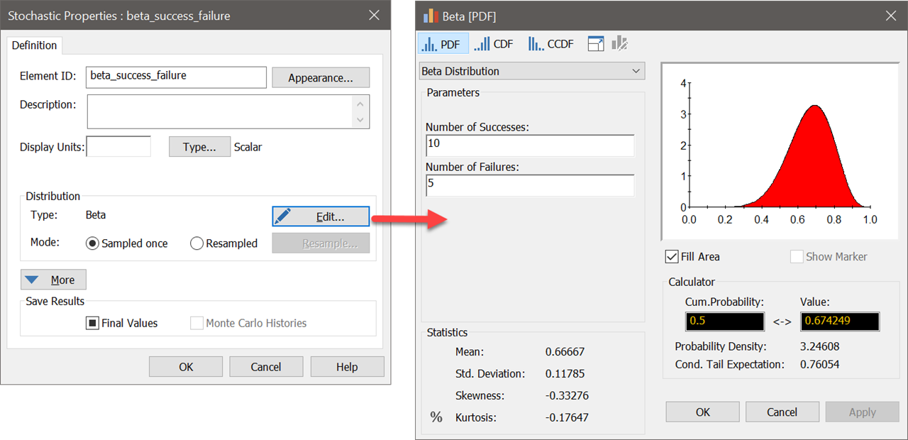
Beta, Generalized Beta, BetaPERT
The Beta distribution represents the uncertainty in the probability of occurrence of an event given observations of the event occurrence in previous experiments.
Given numbers of successes and failures of observations, the beta distribution represents the probability of success on the next trial. You specify the distribution by the number of successes and the number of failures. Values always ranges between 0 and 1.
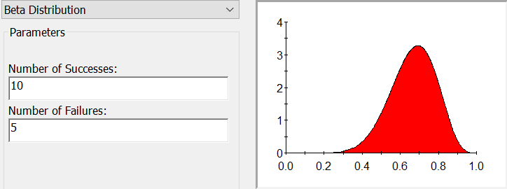
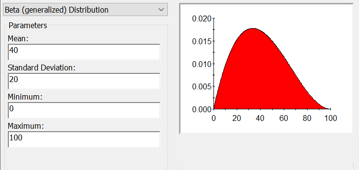
The Generalized Beta distribution provides a flexible way to specify a probability distribution over a particular range. It is commonly used within project management simulations to represent the time to complete a task.
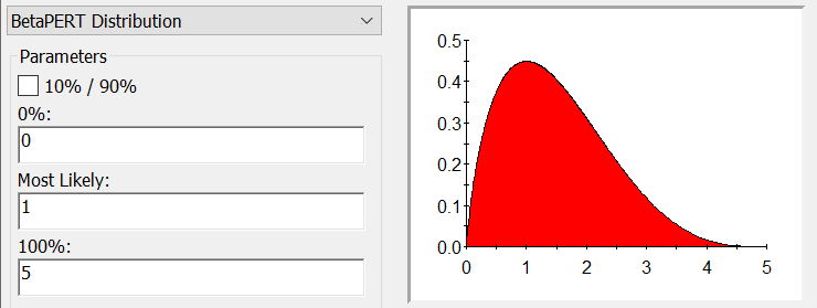
The BetaPERT distribution is a specialized version of the Beta distribution and is often used for project risk analysis.
Binomial, Negative Binomial
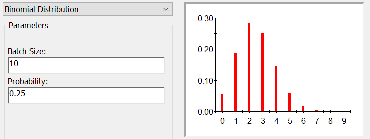
The Binomial distribution describes the probability of a certain number of instances, given a batch size and a probability of occurrence. The binomial distribution can be used to model the number of successes (or failures) from a batch number and a probability of success (or failure).
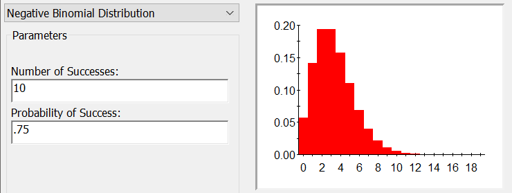
The negative binomial distribution can be used to model the number of failures that occur when trying to achieve a given number of successes. You specify a number of successes and a probability.
Exponential
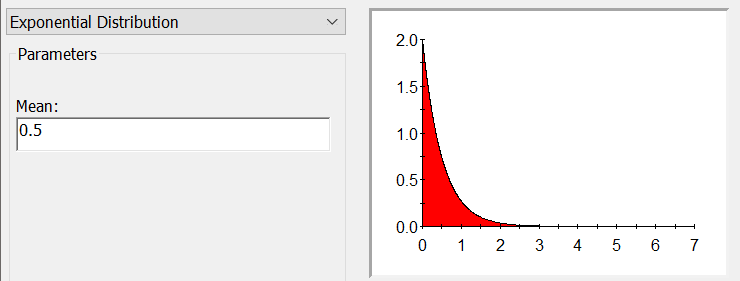
The Exponential distribution is typically used to model the time before the next event, time to complete a task or to reach a milestone.
Extreme Value, Extreme Probability
Extreme distributions model the largest value or the probability of the largest value, given a certain size of sampled results.
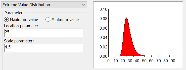
The Extreme Value distribution (also referred to as the Gumbel distribution) describes the maximum (or the minimum) observed values for a variable. It is commonly used to predict the chance of extreme events such as earthquakes or floods.For example, you could use this distribution to specify the probability of the maximum flow rate in a river in a particular year, given the list of maximum values for the past 25 years.
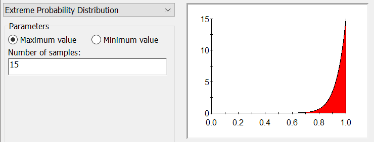
The Extreme Probability distribution is a continuous distribution used to represent the uncertainty in the highest or lowest probability level if any given distribution is sampled N times. As such, the Extreme Probability distribution represents the probability distribution of a probability level, and therefore always ranges between 0 and 1.
Gamma, Truncated Gamma, Pearson Type III
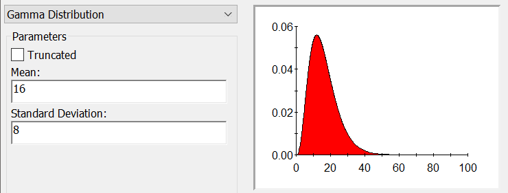
The Gamma distribution represents the time required for the occurrence of a specified number of Poisson events, it is often used to represent the time required to complete a particular task or reach a particular milestone.
The Gamma distribution represents the time required for the occurrence of a specified number of events, i.e., the time to the k-th event, when such an event is modeled by a Poisson process.
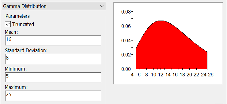
A Gamma distribution can be Truncated, in which case you must specify a Minimum and Maximum value.
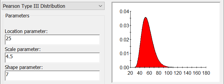
The Pearson Type III distribution is a variation of Gamma distribution that is often used in hydrology. Its is widely used to calculate flood recurrences.
Normal, Truncated Normal, Log-Normal, Truncated Log-Normal
The Normal distribution is the most commonly used probability distribution. It can be used, for example, to represent uncertainties resulting from unbiased measurement error and the value of a sum of other variables.
The normal distribution is specified by a mean and a standard deviation. The linear normal distribution is a bell shaped curve centered about the mean value. The uncertainty of average values, such as a mean value, is often well represented by a normal distribution.
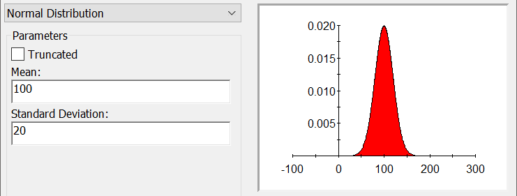
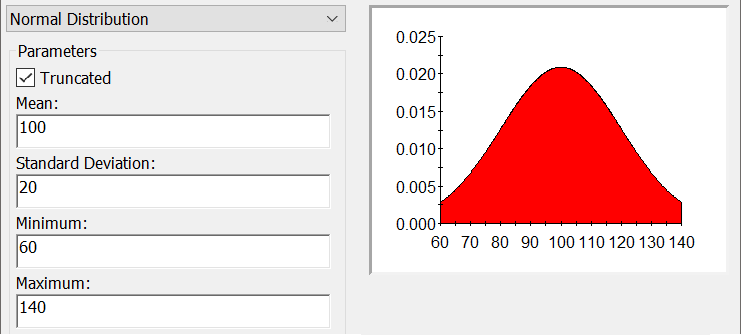
You can truncate the normal distribution (by checking the Truncated box) and specify a Minimum and a Maximum.
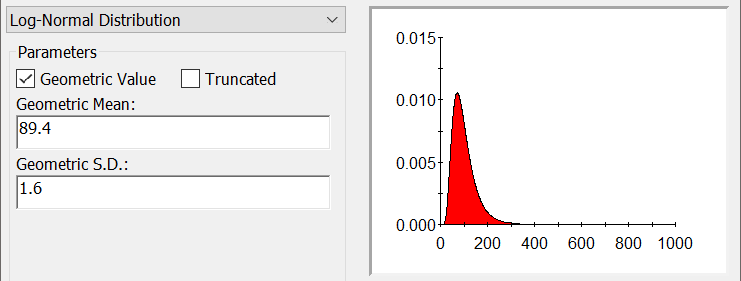
The Log-Normal distribution is used to describe quantities in which the logarithm of the value is normally distributed. The Log-Normal is typically used to represent physical quantities which must be non-negative and are positively skewed. Log-Normal distributions can be entered in two ways: 1) by entering the Geometric Mean and the Geometric S.D.; or 2) by entering the True Mean and the True S.D. If Geometric Value is checked, the former method is used.
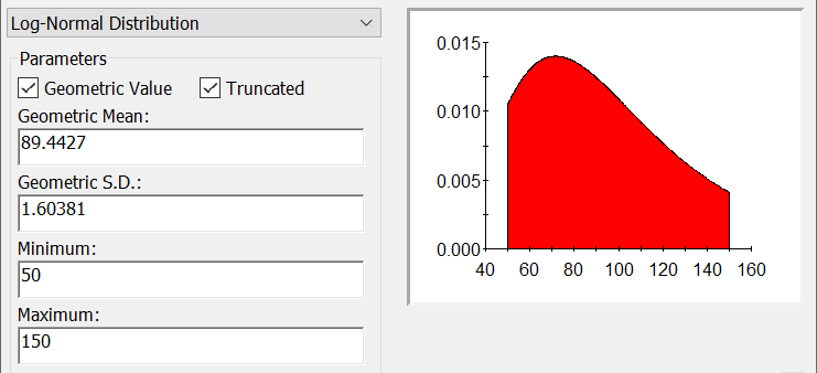
Like the Normal distribution, a Log-Normal distribution can be Truncated. All inputs for a Log-Normal must be positive values.
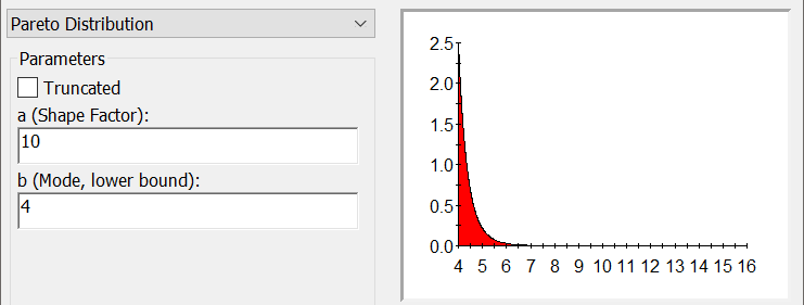
Pareto
The Pareto distribution is widely used to model social, scientific, and other types of observable phenomena, such as traffic patterns in network modeling, the size of insurance claims, and income levels in economic modeling.
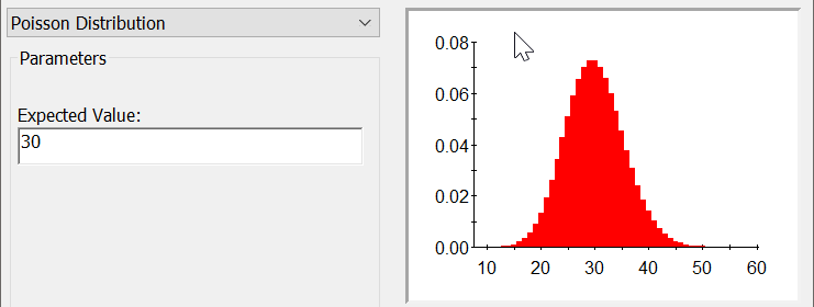
Poisson
The Poisson distribution is used to represent the number of occurrences or instances of a particular event (e.g., number of storms during a year, number of defects in a length of a pipe).
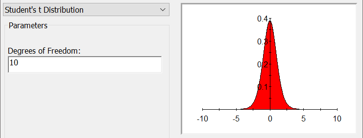
Student's t
The Student’s-t distribution is most commonly used to represent the distribution of an uncertain population mean, given a sample mean and standard deviation.
Triangular, Log-Triangular
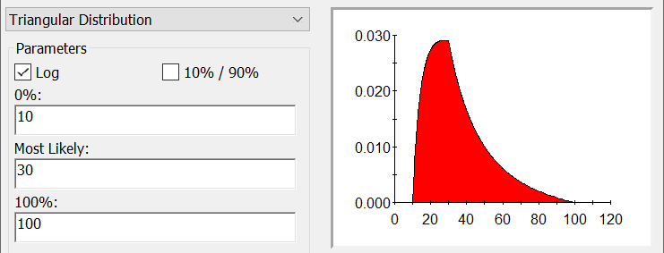
The Triangular distribution is useful in situations where you may have little information about a value, but can provide upper and lower bounds, as well as a "best guess" or most likely value. It is defined by specifying a Minimum, Most Likely, and Maximum value.
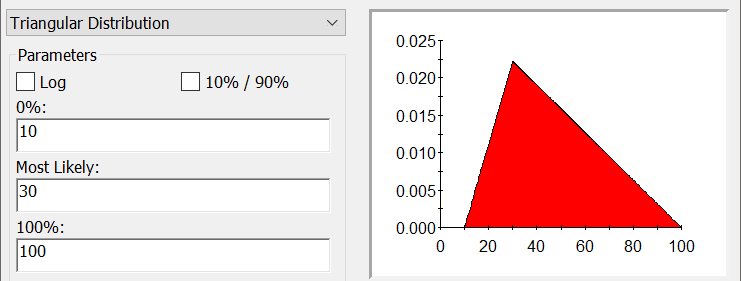
The log-triangular distribution is used when the logarithm of the random variable is described by a triangular distribution. The minimum, most likely and maximum values are specified in linear space.
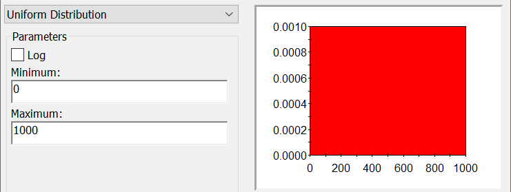
Uniform, Uniform Log
The uniform distribution is specified by a minimum value and a maximum value. Each interval between the endpoints has equal probability of occurrence. This distribution is used when a quantity varies uniformly between two values, or when only the endpoints of a quantity are known.
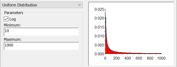
The log-uniform distribution is used when the logarithm of the random variable is described by a uniform distribution. Log-uniform is the distribution of choice for many environmental parameters that may range in value over two or more log-cycles and for which only a minimum value and a maximum value can be reasonably estimated.
Cumulative, Log-Cumulative, Sampled Result, Externally-Defined
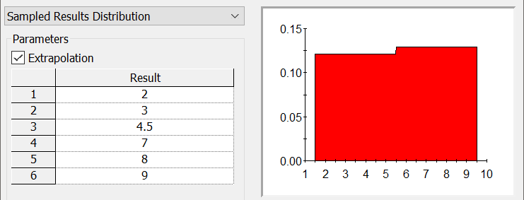
The Sampled Results distribution provides a flexible way to create a non-parametric distribution using a list of sampled (observed) results.Typically, a Sampled Results distribution would only be used with a fairly large number of data points (50 or more).
The Cumulative distribution is used to define custom continuous distributions. You define the distribution by specifying [cumulative probability, value] pairs. By definition, the first cumulative probability specified must be 0 and the last cumulative probability specified must be 1. The Prob. Level and the Value of the pairs cannot decrease as you move downward through the list.
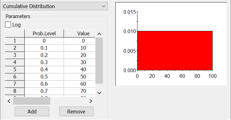
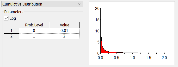
Whereas in a cumulative distribution, the density between values is constant (i.e., the distribution between values is uniform), in a log-cumulative distribution, the density of the log of the value is constant (i.e., the distribution between values is log-uniform). If Log is checked, all Values for the distribution must be positive. Log-Cumulative distributions are often applied to quantities with large (order-of-magnitude) uncertainties.
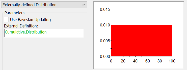
The Externally-defined distribution is a specialized distribution that is defined externally by a Distribution-type output. The primary purpose of this distribution type is to connect a Stochastic to a distribution that has been imported via a Spreadsheet element.
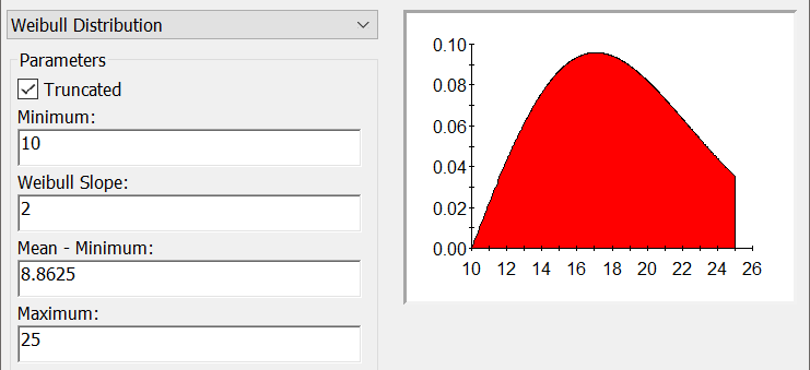
Weibull, Truncated Weibull
The Weibull distribution is applied in a variety of fileds: survival analysis, reliability engineering, modeling dispersion of signals and others. Because the Weibull distribution resembles other statistical distributions, such as the normal or the exponential distribution, it is often used in the field of life data analysis as well.
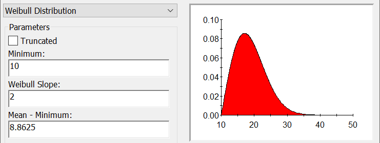
You can truncate the Weibull distribution (by checking the Truncated box) and specify a Minimum and a Maximum.
To Open the Model File:
- Start GoldSim
- Click on the File and select Open Example...
- Browse to General Examples --> Stochastic
- Select the file called Distributions.gsm


Comments
0 comments
Please sign in to leave a comment.