Explicit Separation of Variability from Uncertainty

Example: Separating Uncertainty and Randomness

A new, longer-life lightbulb is proposed for an application that will have one bulb plus two spares. There is a requirement that the combined lives of all three bulbs must exceed 6,000 hours, and you want to know how confident you can be that the requirement will be met.

Because it is a new product there is significant uncertainty about the peformance of the new bulbs. Based on available data you conclude that their failure times will be distributed with a Weibull distribution. However, you are uncertain about the distribution's mean lifetime and the slope factor. You express your uncertainty about the mean as a triangular distribution with a minimum of 2200 hours, most likely value of 2500 hours, and upper bound of 3000 hours. You express your uncertainty about the slope factor of the Weibull distribution as a uniform distribution with a minimum value of 5 and a maximum of 10. Elements "MeanLife" and "Slope" in the parent (outer) model represent these uncertainties. The parent model runs 100 Monte Carlo simulations, and is not dynamic- it has no need to step through time. It simply samples the uncertain Weibull parameters, calls the SubModel to assess the resulting performance, and does some post-processing to display the results.

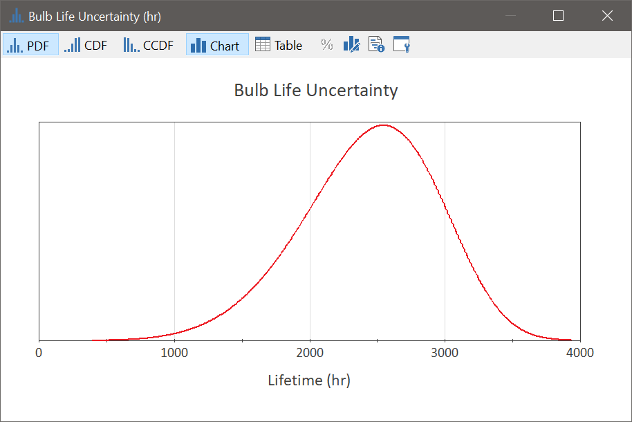
Result element "Bulb Life Uncertainty" displays the lifetime distribution for a single bulb. When the model is in Edit mode it displays the distribution for the mean values of the Weibull parameters. When the model is in Result mode it displays the lifetime distribution based on the last realization of the two uncertain parameters (and hence should be viewed with catution).

The SubModel, "SimulateBulbs", also does 100 Monte Carlo realizations; in each realization it samples and adds up three successive bulb lifetimes. Each time it is called it produces as its output a probability distribution for the total life for three bulbs. This is a purely statistical calculation, and the resulting output distribution is a function of the uncertain mean life and slope factor sampled by the parent model.

Result element "Sum of Three Lifetimes" displays the uncertainties in the lifetime distributions generated by the SubModel. When the model is in Result mode you can view them in a number of different ways:
You can view the entire set of 100 probability distributions for the sum of three bulbs' lifetimes.
You can view any single one of the 100 distributions. 

You can view the distribution of a statistic of each distribution, such as its mean, its 10% quantile, or the probability that it is greater than , equal to, or less than a specified value..
You can view the distribution made up of the combined results for all 10,000 calculations. If you examine this combinded result, you will see that there is a 2.7% chance that the 6,000 hour target wil not be met. However, if you look at the set of 100 distributions you will see that this value might be as high as 12%.

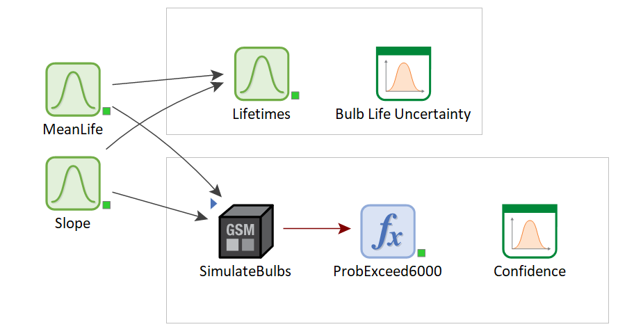
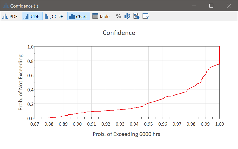
Expression element "ProbExceed6000" takes the lifetime probability distribution returned by the SubModel and calculates the probability that the 6,000-hour target will be exceeded. One such probability is calculated for each realization of the outer model, and the distribution of these probabilities is shown by result element "Confidence". This is the main result of the model- it displays your uncertainty about the probability that the sum of three lifetimes will exceed 6,000 hours. It shows that the probability of exceeding 6,000 hours ranges from 88% to 100%, with a mean value of 97.3%. Does that give you sufficient confidence to select the proposed bulb? Or do you want to have more certainty about your decision?

To Open the Model File:

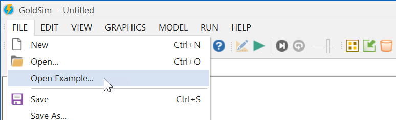
1. Start GoldSim
2. Click on the File and select Open Example...
3. Browse to General Examples --> Submodels
4. Select the file called UncertaintyVariability.gsm